Optimizing Clustering Resolution in Single-Cell Analysis: A Systematic Approach

Clustering is a fundamental step in analyzing high-dimensional single-cell data, helping us understand the relationships between cell populations. One of the most common questions I receive as a data scientist and immunologist is: How do you decide on the clustering resolution? Why choose 0.8 instead of 1.2? The reality is that there is no universal “golden standard” for selecting the best resolution. Instead, the choice is driven by the specific biological question at hand.

For instance, if you’re interested in identifying fine-grained T cell subsets, a lower resolution may not be ideal because it merges biologically distinct populations into a single cluster. A higher resolution, on the other hand, allows for better separation of these subsets. However, finding the optimal resolution is not straightforward—it often requires iterating through multiple clustering resolutions, manually inspecting cluster properties, annotating cell identities, and determining which resolution best aligns with the study’s objectives. This process is both time-consuming and subjective.

To streamline this workflow, I developed a function that automates the exploration of different clustering resolutions. This function systematically evaluates how subclusters emerge from parent clusters as the resolution increases, highlighting the key differentially expressed genes (DEGs) that distinguish them.

How It Works

The function is integrated into Scanpy and is currently available only in Python (apologies to the R/Seurat communities!). Since it’s still in the merge processing stage with Scanpy, I recommend creating a virtual environment before proceeding. The igraph library is required for this function, so make sure to install it via:

pip install igraph
pip install "git+https://github.com/joe-jhou2/scanpy.git@feature-cluster-decision-tree"

Example Workflow

Let’s walk through the example using Scanpy’s PBMC dataset:

import scanpy as sc

# Load the dataset
adata = sc.datasets.pbmc68k_reduced()

# Perform standard preprocessing
sc.pp.normalize_total(adata, inplace=True)
sc.pp.log1p(adata)
sc.pp.pca(adata)
sc.pp.neighbors(adata)
sc.tl.umap(adata)

Note: Do not run sc.tl.leiden(adata) as usual. The following function will automatically run clustering (Leiden) for you.

Step 1: Run the find_resolution function To test multiple clustering resolutions, run:

resolutions = [0.0, 0.2, 0.5, 1.0, 1.5, 2.0]

sc.tl.cluster_resolution_finder(adata, 
                                resolutions=resolutions, 
                                n_top_genes=3, 
                                min_cells=2,
                                deg_mode="within_parent")

‘within_parent’ Comparison: DEGs are identified by comparing sibling clusters that emerged from the same parent. For example, if cluster 1 splits into clusters 4 and 5, the DEGs highlight differences specifically between clusters 4 and 5.

‘per_resolution’ Comparison: DEGs are computed for all clusters at a given resolution, regardless of their parent cluster, providing a broader view of transcriptional differences across the dataset.

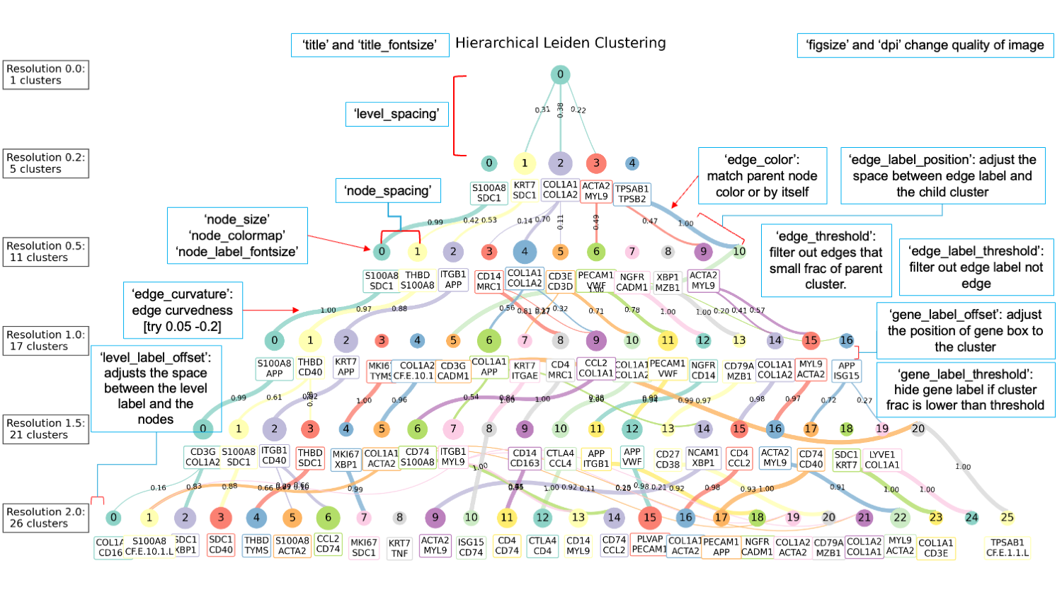
Step 2: Visualize the Hierarchical Clustering Use the cluster_decision_tree function to visualize the hierarchical relationships between clusters at different resolutions:

sc.pl.cluster_decision_tree(adata, resolutions=resolutions, 
                      output_settings = {
                          "output_path": "expected.png",
                          "draw": False,
                          "figsize": (12, 6),
                          "dpi": 300
                          },
                      node_style = {
                          "node_size": 500,
                          "node_colormap": None,
                          "node_label_fontsize": 12
                          },
                      edge_style = {
                          "edge_color": "parent",
                          "edge_curvature": 0.01,
                          "edge_threshold": 0.01,
                          "show_weight": True,
                          "edge_label_threshold": 0.05,
                          "edge_label_position": 0.8,
                          "edge_label_fontsize": 8
                          },
                      gene_label_settings = {
                          "show_gene_labels": True,
                          "n_top_genes": 2,
                          "gene_label_threshold": 0.001,
                          "gene_label_style": {"offset":0.5, "fontsize":8},
                        },
                      level_label_style = {
                          "level_label_offset": 15,
                          "level_label_fontsize": 12
                        },
                      title_style = {
                          "title": "Hierarchical Leiden Clustering",
                          "title_fontsize": 20
                        },
                      layout_settings = {
                          "node_spacing": 5.0,
                          "level_spacing": 1.5
                        },
                      clustering_settings = {
                          "prefix": "leiden_res_",
                          "edge_threshold": 0.05
                        }
                    )

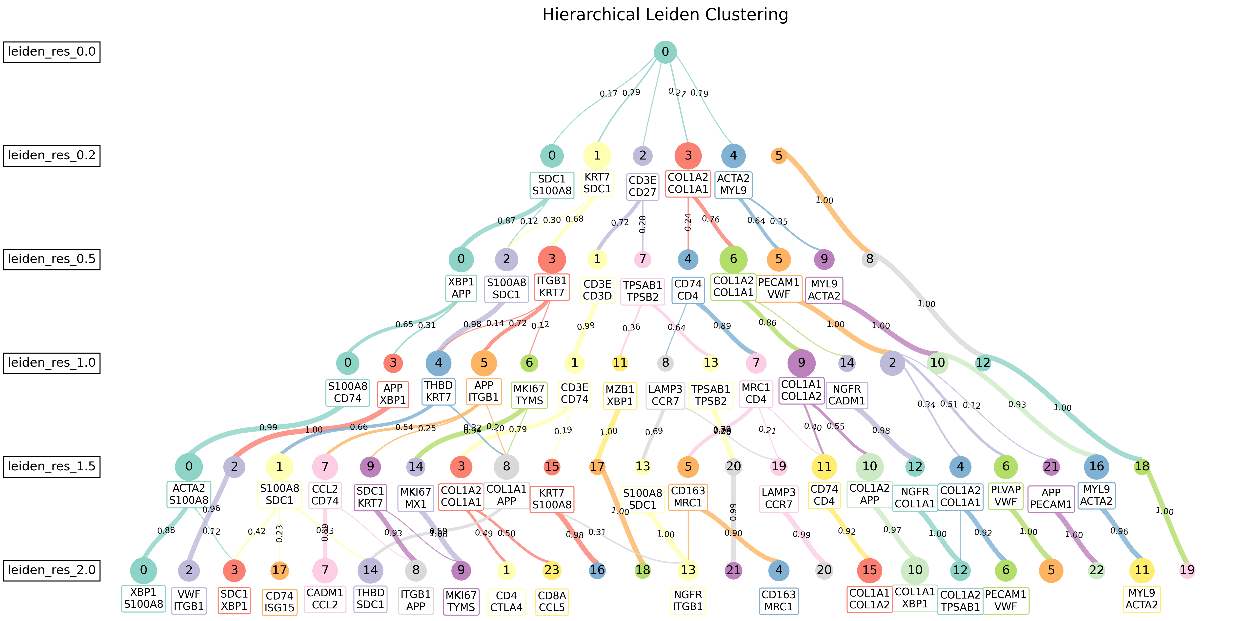
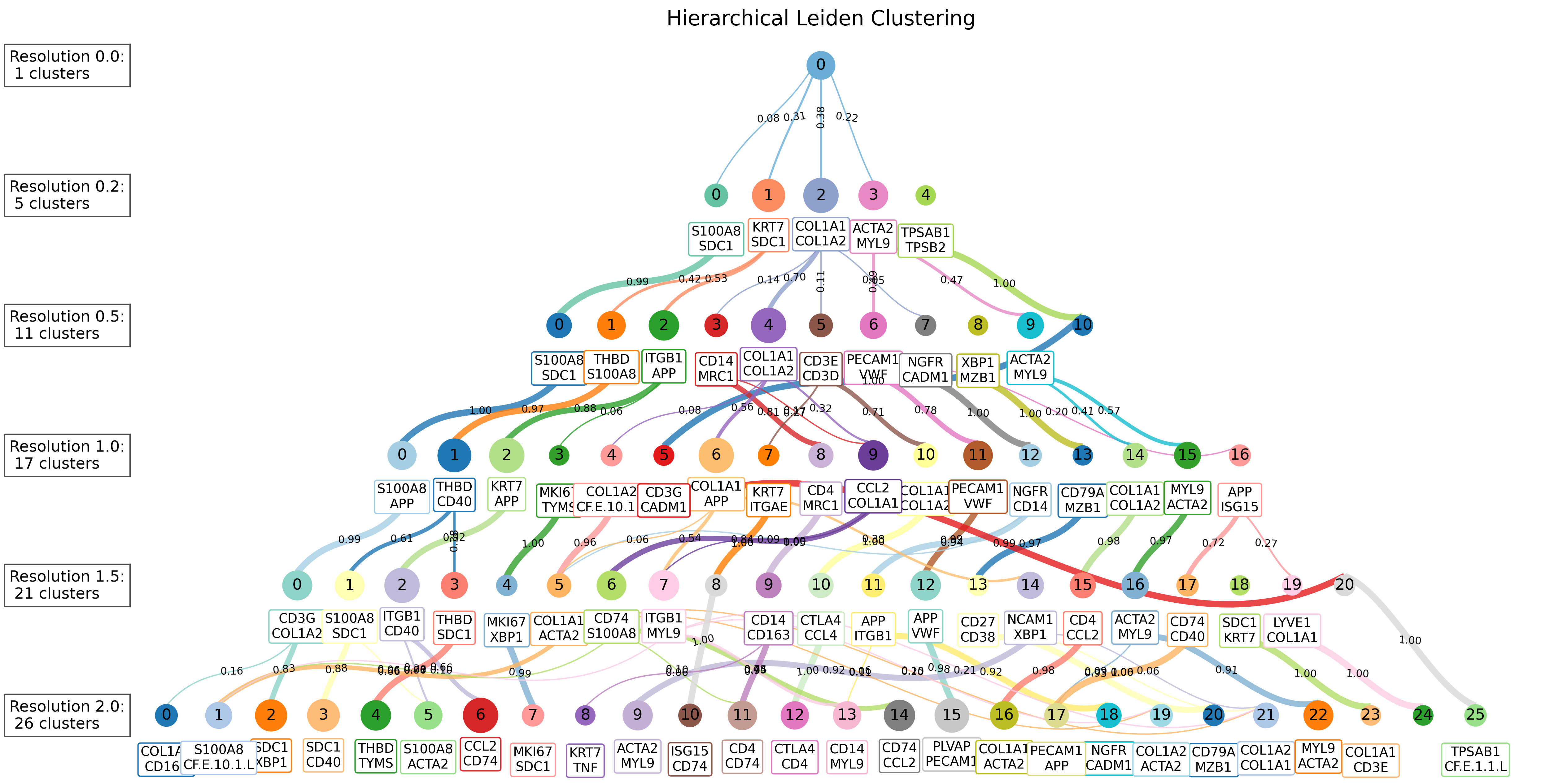
The resulting tree structure provides an intuitive view of how clusters evolve. For example, a parent cluster (e.g., resolution 0.2, cluster 3) may split into multiple child clusters (e.g., resolution 0.5, clusters 6, 9) as the resolution increases. Each node is annotated with the key DEGs that distinguish the subclusters.

Customizing Node Colors The node_colormap parameter accepts various formats for color schemes. If a single color (e.g., ‘red’) is given, the entire level of nodes will be colored that color. If a sequence of color values (e.g., “Set3”) is provided, each node at that level will be assigned a unique color. Here’s an example of different color schemes:

Conclusion While selecting the optimal clustering resolution will always involve some degree of interpretation, this approach makes the process more efficient and data-driven. By automating resolution exploration and systematically tracking DEGs across hierarchical cluster splits, we can make more informed decisions while minimizing manual effort. This workflow is particularly useful for studies that require fine-resolution clustering, such as identifying rare cell subsets in single-cell transcriptomics.

I’d love to hear from others working with single-cell clustering—how do you approach the challenge of resolution selection?